24 May 2026
- 0 Comments
There is nothing quite as frustrating for a variable star observer as pointing your telescope at a bright comparison star only to realize the sky background is glowing like a city streetlamp. You check the weather app; it says clear. But looking up, you see a thick haze of humidity or high-altitude cirrus that turns your sharp stars into fuzzy blobs. In professional astronomy, this night would be scrapped. For amateur astronomers contributing to science through organizations like the American Association of Variable Star Observers (AAVSO), however, we often have no choice but to observe.
This is where understanding atmospheric extinction becomes your best friend. Extinction is the dimming and reddening of starlight as it passes through Earth's atmosphere. When transparency is poor-meaning there is dust, water vapor, or aerosols scattering light-the effect is magnified. Blue light scatters much more easily than red light. If you are using a broadband filter like Johnson V (visual) or even B (blue), your measurements will drift wildly as the target star moves across the sky. The data becomes noisy, unusable, and potentially misleading for researchers studying stellar pulsations.
The solution isn't always to pack up and go home. It is to switch to a red filter, specifically the Johnson R or I band. By observing in longer wavelengths, you bypass the worst of the atmospheric scattering. This guide explains why red filters are superior in poor conditions, how to adjust your workflow, and how to ensure your data remains scientifically valuable despite the gloom.
Why Red Light Penetrates Haze Better Than Blue
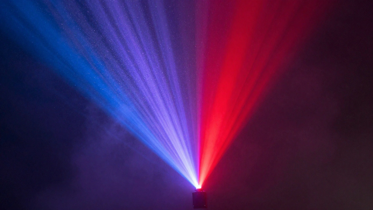
To understand why you should reach for the red filter when the air feels heavy, you need to look at the physics of light scattering. The atmosphere acts like a prism and a sponge combined. Rayleigh scattering, which makes the sky blue during the day, affects shorter wavelengths (blue and violet) significantly more than longer ones (red and infrared). When you add aerosols, pollution, or high humidity to the mix, Mie scattering takes over. This type of scattering is less wavelength-dependent but still favors longer wavelengths for transmission through dense media.
In practical terms, this means that a star’s apparent magnitude changes less dramatically in the red part of the spectrum as it climbs higher in the sky compared to the blue part. Let’s look at the numbers. Under perfect conditions, the extinction coefficient for the V band might be around 0.15 magnitudes per airmass. In poor transparency, that number can spike to 0.4 or even 0.6. However, for the R band, the baseline is lower, often around 0.10, and while it increases with haze, it rarely reaches the chaotic levels seen in V or B. By shifting your observation window to the red, you reduce the "noise" introduced by the atmosphere itself.
| Filter Band | Peak Wavelength (nm) | Good Transparency k-value | Poor Transparency k-value | Stability Rating |
|---|---|---|---|---|
| B (Blue) | 445 | 0.25 | > 0.80 | Poor |
| V (Visual) | 551 | 0.15 | 0.40 - 0.60 | Moderate |
| R (Red) | 658 | 0.10 | 0.20 - 0.35 | Good |
| I (Infrared) | 806 | 0.07 | 0.15 - 0.25 | Excellent |
Note that these values vary by location. Observers in dry, high-altitude deserts will see different coefficients than those in humid coastal cities like Portland. The key takeaway is the relative stability: R and I bands provide a flatter slope, making differential photometry more reliable when the atmosphere is turbulent.
Choosing the Right Red Filter for Your Setup
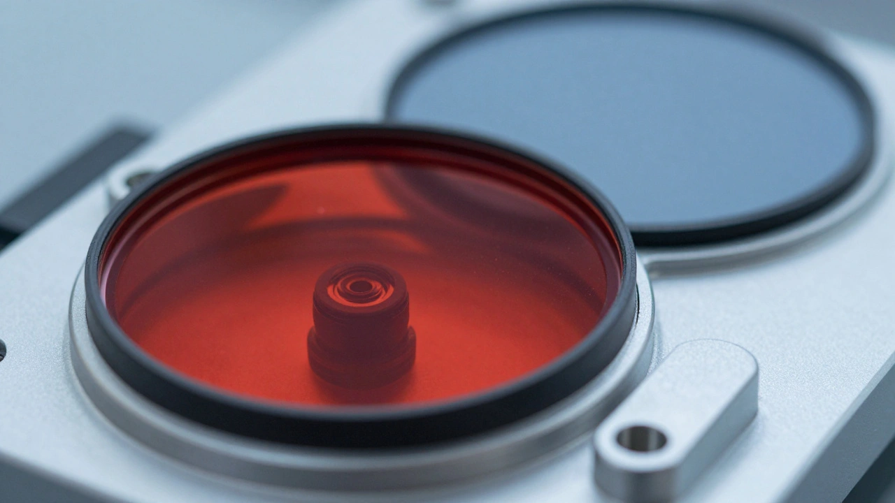
Not all red filters are created equal. In the context of variable star photometry, precision matters. You want a filter that matches standard astronomical systems so your data can be compared with professional datasets. The two primary choices are the Johnson-Cousins R and I filters.
The Johnson R filter is the most common starting point for amateurs dealing with haze. It has a peak transmission around 658 nanometers. It offers a good balance between reduced extinction and detector sensitivity. Most modern CMOS and CCD sensors have decent quantum efficiency in this range, meaning you don’t need excessively long exposures to get a clean signal-to-noise ratio. If you are using a monochrome camera, an R filter is essential. If you are using a color camera, you can extract the red channel, but dedicated filters usually offer sharper cutoffs and better rejection of unwanted wavelengths.
The Cousins I filter goes further into the near-infrared, peaking around 806 nanometers. This is the ultimate weapon against transparency issues. Because it sits almost entirely outside the visible spectrum, it is largely immune to the blue-scattering effects of aerosols. However, there are trade-offs. Many older CCD cameras have very low sensitivity in the I band unless they are specifically cooled and modified. Additionally, thermal noise becomes a bigger factor in the infrared. If your camera runs hot, your dark frames will be noisy, and subtracting them becomes critical. For most general-purpose variable star work in poor seeing, the R filter is the sweet spot. Save the I filter for targets that are extremely red, like M-type giants, or when the transparency is absolutely terrible.
Adjusting Your Photometric Workflow
Switching to a red filter isn't just about changing the wheel position on your filter drawer. It requires adjustments to your exposure times and your comparison star selection. Here is how to adapt your process to maintain data integrity.
- Recalculate Exposure Times: Red filters transmit less total light than broad-band visual filters if your sensor is not optimized for IR. Start with a test image. Aim for a peak ADU (Analog-to-Digital Unit) value of 50-70% of your full well capacity for your brightest comparison star. If you are used to 30-second exposures in V, you might need 45-60 seconds in R. Don't guess; check the histogram.
- Select Appropriate Comparison Stars: Ensure your comparison stars are within 2 magnitudes of your target in the R band. Color terms become significant if your comparison stars have vastly different spectral types than your target. In poor transparency, this error is amplified. Use catalogs like the AAVSO International Database to find R-band magnitudes for your field stars.
- Monitor the Sky Background: Even in red light, light pollution and moon glow affect your measurements. Measure the sky background in empty regions of your frame. If the sky background is rising rapidly due to passing clouds or increasing humidity, note the time. Consistent sky background subtraction is vital for aperture photometry.
- Check for Flat Field Errors: Dust motes and vignetting appear differently in red light. Take fresh flat frames whenever you change filters. A flat field taken in V will not correct for optical aberrations in R. Neglecting this introduces systematic errors that mimic variability.
Handling Data Reduction and Calibration
Once you have captured your images, the real work begins. Software like AstroImageJ, Iris, or Python-based pipelines using Astropy will handle the math, but you need to know what parameters to trust. The biggest enemy in poor transparency is the assumption that the atmosphere is stable. It isn't.
When performing differential photometry, you measure the flux of your target star relative to one or more comparison stars. In ideal conditions, the ratio remains constant regardless of airmass. In poor transparency, the ratio may drift slightly if the comparison stars are at significantly different altitudes or if their colors differ greatly from the target. This is known as the "color term."
To mitigate this, use multiple comparison stars. Average their ratios. If one star shows a sudden jump in brightness while others remain steady, discard that measurement-it was likely obscured by a thin cloud wisp. Always plot your data against airmass before submitting. If you see a strong linear trend in your residuals (the difference between measured and expected magnitude) correlated with airmass, your extinction correction is off. In red filters, this slope should be minimal. If it’s steep, re-evaluate your sky subtraction or check for saturation in your comparison stars.
Remember to log the conditions. Note the transparency qualitatively (e.g., "hazy," "cirrus present") and quantitatively if possible (e.g., "extinction coefficient estimated at 0.25 mag/airmass"). This metadata helps researchers weight your data appropriately. A dataset labeled "poor transparency, R-band" is still valuable because it provides coverage during nights when other observers couldn't see. It fills gaps in light curves, especially for short-period variables.
When to Stop Observing
While red filters extend your usable observing window, they are not magic. There are limits. If the seeing is so poor that stars are dancing violently across pixels, your centroiding algorithms will fail, leading to scatter in your photometry. If the transparency is so bad that your faintest comparison stars disappear into the noise floor, you cannot establish a reliable baseline.
A practical rule of thumb: if your signal-to-noise ratio (SNR) for your comparison stars is below 20, your error bars will be too large for precise scientific contribution. In such cases, it is better to wait. However, for long-period variables like Mira stars, where changes happen over weeks, a single noisy point in R-band is often preferable to no point at all. Just flag the uncertainty in your submission notes.
Ultimately, the goal is consistency. Whether you are tracking the pulsation of a Cepheid or the erratic outbursts of a dwarf nova, providing continuous coverage is key. Using red filters wisely allows you to contribute meaningful data even when the sky fights back. It transforms a wasted night into a productive session, ensuring that the story of the variable star continues to be told, one photon at a time.
Can I use a red filter on a color camera?
Yes, but it is not ideal. Color cameras have a Bayer filter matrix that splits light into red, green, and blue channels. While you can extract the red channel, the effective bandwidth is narrower and less defined than a dedicated Johnson R filter. This can introduce color terms and reduce throughput. For serious photometry, a monochrome camera with a dedicated filter wheel is recommended. If you must use a color camera, ensure your software correctly debayers and extracts the red channel without mixing in green data.
How do I calculate the extinction coefficient for my site?
You can estimate the extinction coefficient by observing a standard star field at different airmasses. Plot the instrumental magnitude against airmass. The slope of the resulting line is your extinction coefficient (k). Do this regularly, as k varies with humidity, season, and local pollution. Many photometry software packages include tools to automate this calculation. Aim to perform this calibration under both good and poor conditions to understand the range of variation at your site.
Is I-band photometry worth the effort for beginners?
For most beginners, sticking to V and R bands is sufficient. I-band requires careful handling of thermal noise and often specialized equipment. However, if you observe cool stars (M-types) or face persistent high-humidity conditions, investing in an I filter can yield cleaner data. Start with R-band to master the basics of differential photometry in non-standard conditions before moving to the complexities of near-infrared imaging.
Does light pollution affect red filters less?
It depends on the source. Sodium-vapor streetlights emit strongly in the yellow-orange part of the spectrum, which can bleed into the R band. LED lights, which are becoming more common, have broader spectra. Generally, red filters reject some of the blue-rich skyglow from urban areas, but they do not eliminate it. Always measure and subtract the sky background accurately. In remote locations, R-band observations are cleaner, but in cities, you must be vigilant about background subtraction.
How does humidity specifically impact photometry?
Humidity increases atmospheric opacity, particularly in the infrared, but it also enhances Mie scattering in the visible spectrum. High humidity leads to rapid fluctuations in transparency, causing "seeing" to degrade and star images to twinkle intensely. This results in higher scatter in your photometric measurements. On humid nights, increase your integration time slightly to average out the turbulence, and rely heavily on R-band filters to minimize the extinction variations caused by water vapor.