16 Sep 2026
- 0 Comments
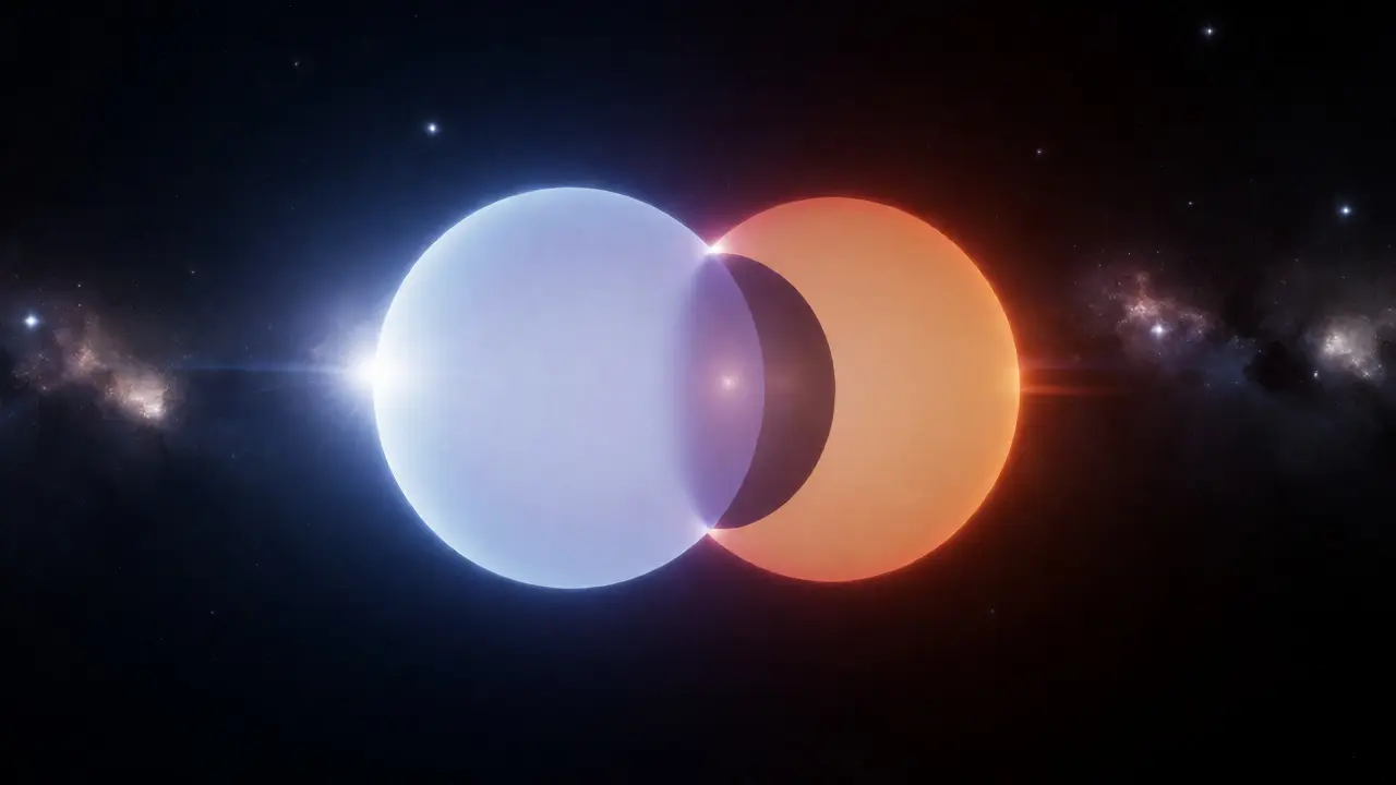
Imagine watching a star dim by half its brightness in just a few minutes, then slowly return to normal. You aren't seeing a cloud pass over the lens or a sensor glitch. You are witnessing two stars orbiting each other, with one physically blocking the light of the other. This phenomenon defines Eclipsing Binary Variables, a specific class of variable stars where the observed brightness changes due to mutual eclipses rather than intrinsic pulsations or eruptions. For amateur astronomers and professional photometrists alike, these systems offer a rare glimpse into stellar mechanics that we can measure directly from Earth.
If you have ever looked through a telescope at a steady point of light and wondered if it was truly constant, you might be missing out on some of the most dynamic objects in the night sky. Eclipsing binaries are not just pretty lights; they are cosmic laboratories. By measuring exactly how much light is blocked and for how long, we can calculate the mass, radius, and temperature of stars millions of miles away without ever leaving our backyard. But observing them requires a different approach than tracking planets or galaxies. It demands patience, precise timing, and an understanding of what makes the light curve tick.
What Exactly Is an Eclipsing Binary?
At its core, an eclipsing binary is a pair of stars bound by gravity, orbiting a common center of mass. The key feature here is orientation. We must view this system almost edge-on from our perspective on Earth. If the orbital plane were tilted toward us like a coin lying flat on a table, we would see both stars simultaneously all the time, and their combined brightness would remain steady. But when the plane is aligned with our line of sight, one star passes in front of the other periodically.
This alignment creates two distinct types of dips in brightness during each orbital cycle:
- Primary Eclipse: This occurs when the brighter star is obscured by the fainter companion. Because a large amount of light is blocked, the drop in magnitude is significant and sharp.
- Secondary Eclipse: This happens when the fainter star passes behind the brighter one. Less total light is lost, so the dip is shallower and often harder to detect visually.
The period between these events tells us the orbital period of the system. Some binaries zip around each other in hours, while others take years. For observers, shorter periods mean more frequent chances to catch an eclipse, making them ideal targets for learning photometry.
Why Measure Light Curves Instead of Just Looking?
You might ask, "Can I just watch it through my eyepiece?" Sometimes, yes. Famous examples like Algol (Beta Persei) dim enough to be noticed by the naked eye over several nights. However, visual estimation is subjective and prone to error. Human eyes cannot reliably distinguish small changes in brightness, especially against the background sky glow or atmospheric turbulence.
To get real scientific value, we generate a Light Curve, which is a graph plotting a star's brightness against time. This data visualization reveals the shape of the eclipse, the depth of the dip, and the duration of totality. These details allow astronomers to derive physical properties of the stars involved. For instance, the width of the eclipse correlates with the size of the stars relative to their orbital distance. A wider dip suggests larger stars or a slower orbital velocity.
Modern technology has democratized this process. What once required expensive photoelectric photometers can now be achieved with consumer-grade DSLR cameras, dedicated CCDs, or even CMOS sensors found in modern astrophotography rigs. Software like AstroImageJ or VStar allows you to reduce raw images into usable light curves right on your laptop.
Choosing Your First Target
Not all eclipsing binaries are created equal. When starting out, you want targets that are bright enough to yield good signal-to-noise ratios but not so bright that they saturate your camera sensor instantly. You also want predictable ephemerides-timetables that tell you when the next eclipse will occur.
| Star Name | Constellation | Magnitude Range | Period (Days) | Difficulty Level |
|---|---|---|---|---|
| Algol (β Per) | Perseus | 2.1 - 3.4 | 2.87 | Beginner |
| W UMa | Ursa Major | 7.7 - 8.5 | 0.33 | Intermediate |
| YY Gem | Cancer | 8.7 - 9.3 | 0.81 | Advanced |
| RY Cha | Chamaeleon | 10.0 - 10.6 | 0.90 | Expert |
Algol is the classic choice. Known as the "Demon Star," it dims noticeably every 2.87 days. Its brightness change is dramatic enough that early civilizations associated it with bad omens. Today, it serves as a benchmark for testing photometric equipment. If your setup can accurately capture Algol’s primary eclipse, it is likely calibrated correctly for fainter targets.
W Ursae Majoris (W UMa) represents a different beast entirely. It is a contact binary, meaning the two stars are so close they share a common envelope of gas. Their light curve looks different-smooth and sinusoidal rather than having sharp, flat-bottomed eclipses. Observing W UMa teaches you about continuous variation versus discrete events.
Setting Up for Success: Equipment and Technique
You do not need a 16-inch Dobsonian to observe eclipsing binaries effectively. In fact, smaller apertures often work better because they provide a wider field of view, allowing you to include comparison stars in the same frame. Comparison stars are non-variable stars near the target that serve as reference points. By comparing the brightness of your target to these stable references, you cancel out atmospheric extinction and instrumental drift.
Here is a practical checklist for setting up your observation session:
- Check the Ephemeris: Use resources like the AAVSO (American Association of Variable Star Observers) website to find predicted eclipse times. Aim to start observing at least one hour before the predicted minimum to capture the ingress (the falling part of the curve).
- Select Comparison Stars: Choose three nearby stars with similar colors to your target. Color matters because blue filters react differently to red stars than green ones. If possible, use standard photometric filters (V-band) to match historical data.
- Defocus Slightly: Unlike deep-sky imaging where sharp focus is king, photometry benefits from slightly defocused stars. This spreads the light across more pixels, reducing errors caused by tiny pointing inaccuracies or atmospheric scintillation.
- Keep Exposure Times Constant: Do not adjust exposure settings during the sequence unless absolutely necessary. Consistency is critical for accurate relative brightness measurements.
Timing is everything. Record the exact UTC time of each image. Even a minute off can skew the phase plot, shifting the eclipse features left or right on your graph. Most modern cameras embed this timestamp in the EXIF data, but double-check your camera clock against a reliable source like NIST before starting.
Analyzing the Data: From Pixels to Physics
Once you have collected a series of images covering the eclipse, the real work begins. You load these files into photometry software. The software measures the total flux (light intensity) within a circular aperture around the target star and subtracts the background sky brightness. It does the same for your comparison stars.
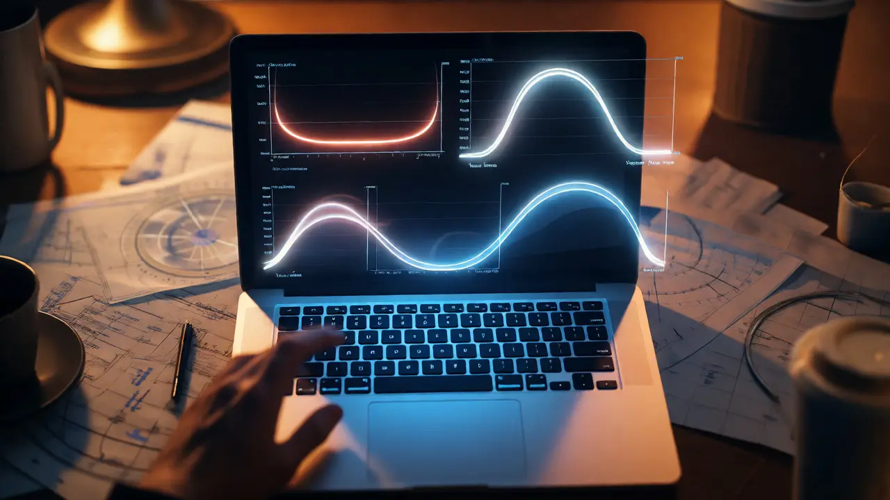
The software then calculates the ratio of the target's flux to the average flux of the comparison stars. Plotting this ratio against time produces your light curve. Look for specific features:
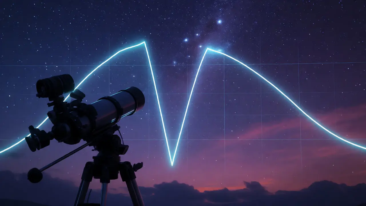
- Flat Bottom: Indicates a total eclipse where the smaller star completely covers the disk of the larger one.
- V-Shaped Dip: Suggests a partial eclipse or grazing geometry where no totality occurs.
- Out-of-Eclipse Variation: Small bumps outside the main dip might indicate spots on the stellar surface or ellipsoidal effects (where the stars distort each other's shapes due to tidal forces).
Interpreting these shapes helps classify the system. Detached binaries (stars well separated) show sharp, square-bottomed eclipses. Semi-detached systems (one star filling its Roche lobe) show rounded bottoms. Contact binaries show smooth, wave-like curves. By fitting theoretical models to your observed light curve, you can estimate the inclination of the orbit and the radii of the stars.
Common Pitfalls and How to Avoid Them
Even experienced observers run into trouble. Cloud cover is the obvious enemy, but subtle issues can ruin data quality. One common mistake is using comparison stars that are actually variable themselves. Always check databases like VSX (Variable Star Index) to ensure your reference stars are listed as "non-variable" or "constant." Another issue is saturation. If your target is too bright, the pixel values hit the maximum limit, clipping the data. You lose information about how much brighter it actually is. Mitigate this by using neutral density filters or shorter exposures.
Atmospheric conditions also play a role. High humidity can cause condensation on optics, scattering light and lowering contrast. Dew heaters are essential for long sessions, especially in coastal areas like Portland where moisture hangs heavy in the air. Furthermore, moonlight can wash out fainter targets. Plan your observations during new moon phases or when the moon is below the horizon for best results with magnitude 8+ stars.
Beyond Visual: Contributing to Science
Why bother with all this effort? Because amateur data matters. Professional telescopes like TESS (Transiting Exoplanet Survey Satellite) monitor huge swaths of sky but often lack the temporal resolution to follow up on interesting transient events quickly. Ground-based observers fill this gap. Organizations like the AAVSO maintain global networks of contributors who submit light curves regularly.
Your observations can help refine orbital parameters, discover third bodies in the system via timing variations, or even detect exoplanets transiting one of the stars in the binary. Every valid light curve adds to the collective understanding of stellar evolution. It transforms passive stargazing into active participation in astrophysical research.
Do I need a telescope to observe eclipsing binaries?
No, not necessarily. Bright targets like Algol can be monitored with binoculars or even the naked eye under dark skies. However, a telescope or telephoto lens attached to a camera is required for photometric precision and for observing fainter systems.
How many images do I need for a good light curve?
There is no fixed number, but generally, taking an image every 1-5 minutes during the eclipse event is recommended. More frequent sampling provides higher resolution of the eclipse shape. Aim for at least 20-30 points per hour to capture the ingress and egress smoothly.
What is the difference between an eclipsing binary and an exoplanet transit?
The mechanism is similar-a body passing in front of a star-but the scale differs. In eclipsing binaries, the object blocking the light is another star, causing deep dips (often >0.1 magnitudes). In exoplanet transits, the object is a planet, causing shallow dips (typically <0.02 magnitudes). Detecting exoplanets requires much higher precision equipment.
Which software should I use for reduction?
AstroImageJ is free, powerful, and widely used by the AAVSO community. VStar is another excellent option for managing light curve data. Both support differential photometry and export formats compatible with modeling tools like JKTEBOP.
Can clouds ruin my entire observation session?
Clouds interrupt data collection but don't necessarily ruin the session if you have gaps. You can still analyze the clear portions. However, thin cirrus clouds can introduce noise by varying transparency unpredictably. It is best to avoid observing through thin clouds if high precision is required.