16 Aug 2026
- 0 Comments
Staring at a bright star through your CMOS camera and seeing its brightness flicker? That’s not necessarily the star changing. It’s likely your atmosphere, your focus, or your calibration failing you. For beginners tackling variable stars, the difference between a usable data point and noise often comes down to understanding how light interacts with your sensor before it even hits the pixels.
Photometry isn’t just about taking pictures; it’s about measuring the amount of light accurately. When using modern CMOS sensors, you have high sensitivity but also specific artifacts like blooming and non-linear response that can ruin your measurements if ignored. This guide walks you through the exact workflow to get reliable data and the pitfalls that trip up almost every new observer.
Understanding Your Sensor: The Foundation of Accuracy
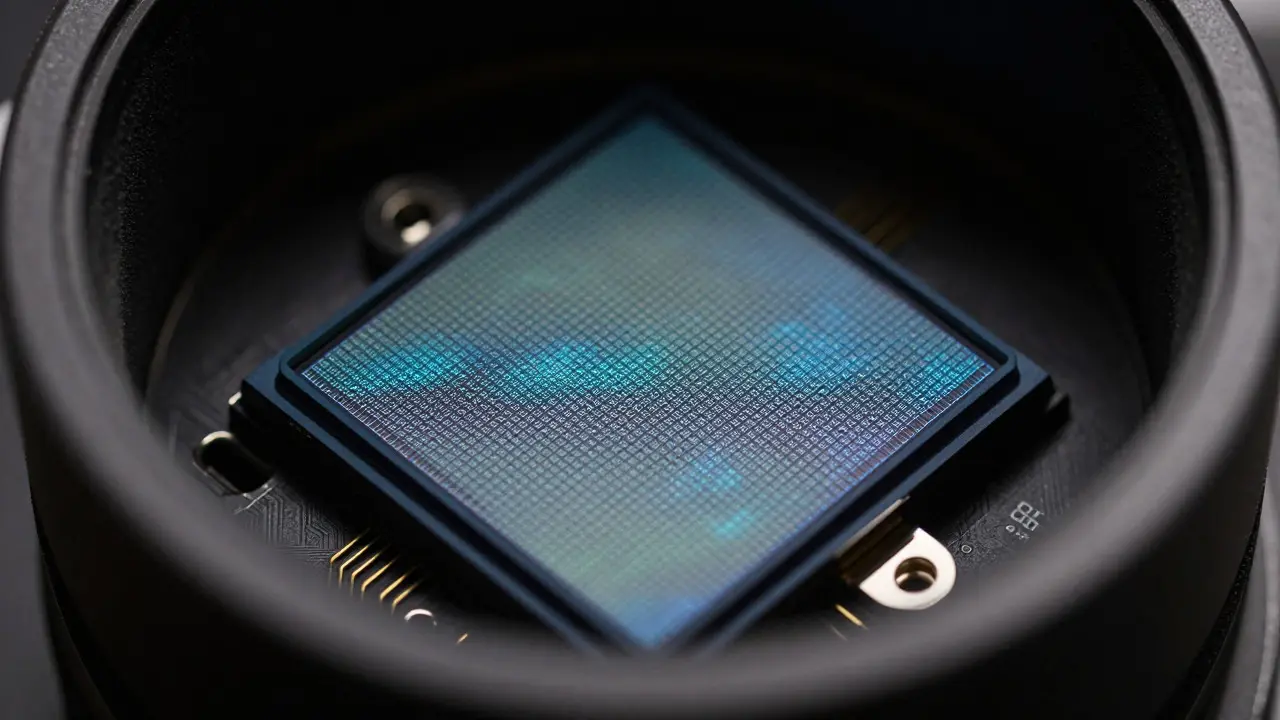
Before you point your telescope at Betelgeuse or Algol, you need to know what your hardware is actually doing. A CMOS Camera is a digital imaging sensor that converts photons into electrical signals directly at each pixel site. Unlike older CCDs, which read out charge sequentially, CMOS cameras read out faster and generate less heat, making them ideal for uncooled use in many amateur setups. However, this speed comes with a trade-off: read noise and fixed pattern noise (FPN) are more pronounced if not managed correctly.
The key attribute here is the Full Well Capacity. This is the maximum number of electrons a single pixel can hold before it saturates (blooms). If your target star exceeds this limit, the data is useless because the peak flux no longer correlates linearly with brightness. Most consumer-grade CMOS cameras used in astronomy have a full well capacity between 10,000 and 50,000 electrons per pixel. You must ensure your brightest reference stars stay below this threshold to maintain linearity.
The Essential Photometric Workflow
A robust photometric session follows a strict sequence. Skipping steps here is the fastest way to introduce systematic errors that mimic stellar variability.
- Dark Frames: Capture these with the same exposure time as your science frames but with the lens cap on. CMOS sensors have significant thermal noise even at low temperatures. Subtracting darks removes this bias.
- Bias Frames: These are very short exposures (usually under 1 millisecond) that capture the electronic offset of the sensor. They are crucial for correcting the pedestal level added by the camera’s analog-to-digital converter.
- Sky Flats: This is where most beginners fail. You need to illuminate the sensor uniformly with twilight sky or an artificial dome flat. Sky flats correct for vignetting, dust motes, and pixel-to-pixel gain variations. Without proper flats, a star moving across the field will appear to change brightness simply because it moved from a 'darker' part of the image to a 'brighter' part.
- Science Frames: Finally, take your images of the variable star and comparison stars. Use consistent filter settings (typically Johnson-Cousins V-band or B-band) to isolate specific wavelengths.
Remember, the order matters. Darks and biases should be taken at the start and end of your session to account for any temperature drift. Flats should be taken when the sky brightness matches the conditions during your science run, or you must normalize them carefully.
Common Pitfalls That Ruin Data
Even with perfect equipment, atmospheric turbulence and processing errors can create false positives. Here are the three biggest traps for beginners.
- Aperture Correction Errors: As a star gets brighter, its halo spreads further due to atmospheric seeing. If you use a fixed small aperture, you miss the outer light. If you use a huge fixed aperture, you include too much background sky noise. The solution is Aperture Correction: plotting the measured magnitude against the size of the measurement aperture and finding the optimal radius where the curve flattens. Most software packages do this automatically, but you must verify it works for your specific seeing conditions.
- Non-Linearity and Saturation: If a comparison star is too bright, its core pixels hit zero value (saturation). Once saturated, the relationship between electron count and brightness breaks down. Always check your histogram. If the peak of the star’s profile touches the bottom axis, reduce your exposure time.
- Atmospheric Extinction: The lower a star is in the sky, the more atmosphere its light passes through, dimming it. This effect depends on the star’s altitude (airmass). To mitigate this, keep your targets above 45 degrees elevation if possible, or apply extinction corrections based on local weather data. Ignoring this makes a star look fainter simply because it set, not because it faded.
Choosing Comparison Stars
You cannot measure a variable star in isolation. You need stable references. The best practice is to select 3-5 comparison stars within the same field of view. These stars should be:
- Unvariable (check databases like SIMBAD or VSX to confirm).
- Similar in brightness to your target (within 1-2 magnitudes) to avoid saturation issues.
- Distributed around the target to average out local seeing fluctuations.
If you only have one comparison star, your error bars will be large. If your comparison stars are themselves variables, your data is compromised. Always cross-reference your chosen standards with published catalogs before starting your night.
Data Reduction and Analysis
Once you have your calibrated images, you move to analysis. Software like AstroImageJ, IRAF, or dedicated photometry tools like DiffImg allow you to extract flux values. The goal is to calculate the relative magnitude of your target compared to the average of your comparison stars.
| Filter | Wavelength Range (nm) | Best For | Limitation |
|---|---|---|---|
| Johnson V (Visual) | 550 nm | Cepheids, RR Lyrae | Requires narrowband filters for precision |
| Johnson B (Blue) | 440 nm | Hot stars, eclipsing binaries | More affected by atmospheric scattering |
| Clear/Broadband | 400-700 nm | Rapid changes, supernovae | Poor color separation, higher noise |
When plotting your results, look for scatter. If your points jump randomly by more than 0.05 magnitudes, your calibration is likely unstable. Consistent scatter indicates good technique. Over time, you’ll see the true pulsation period emerge from the noise.
Practical Tips for Your First Session
Start simple. Don’t try to monitor a fast pulsator like Delta Scuti on your first night. Choose a slow variable like Mira or a well-known eclipsing binary like Algol. Use a moderate focal length so your field of view includes several comparison stars. Keep your exposure times short enough to prevent saturation but long enough to minimize read noise (typically 10-60 seconds depending on your camera gain). Finally, log everything: date, time, airmass, seeing conditions, and filter used. This metadata is as important as the data itself when publishing your results.
Do I need a cooled CMOS camera for photometry?
Not necessarily. While cooling reduces thermal noise, a good uncooled CMOS camera with proper dark frame subtraction can achieve photometric precision of 0.01 to 0.05 magnitudes. Cooling becomes critical if you plan to take very long exposures (over 2 minutes) or observe in hot environments where sensor temperature fluctuates significantly.
What is the minimum number of comparison stars I should use?
Three is the practical minimum. Using three or more allows you to calculate the standard deviation of the comparison stars themselves. If the spread among your comparisons is larger than your target’s variation, your measurement is unreliable. Ideally, you want five to seven stars to average out individual atmospheric scintillation effects.
How do I handle clouds passing over my target?
If a cloud partially covers the field, discard those frames unless you can reliably mask the clouded region. If the entire field dims uniformly, you may still use the data if you apply a global scaling factor, but it introduces uncertainty. It is better to pause observing and wait for clear skies rather than risk introducing systematic errors that are hard to remove later.
Can I use smartphone photos for variable star monitoring?
Yes, for rough monitoring. Smartphone cameras have automatic white balance and HDR processing that distort linear relationships. To use them effectively, disable all auto-corrections, shoot in RAW format, and treat the data as semi-quantitative. Precision will be lower (around 0.1 to 0.2 magnitudes), but trends can still be valuable for citizen science projects.
What is the role of airmass in photometric accuracy?
Airmass represents the path length of light through Earth's atmosphere. As airmass increases (star gets lower), light is scattered and absorbed more. This causes the star to appear fainter and redder. For precise work, you must either restrict observations to low airmass (< 1.5) or apply mathematical extinction corrections derived from simultaneous observations of standard stars at different altitudes.